Teaching a Model to Read Financial Regulations

A financial regulation rarely belongs to exactly one category. A single provision on digital transactions can be relevant to e-money, payment gateways, and credit cards at the same time. In compliance auditing, that detail is the whole game: to estimate how many person-days an audit will take, you first have to identify every regulation that touches a client's operational scope. Today that means a human reading dense, highly technical regulatory documents from Indonesia's Financial Services Authority (OJK) and Bank Indonesia (BI) — a slow and expensive process.

This note is a write-up of a paper I worked on with Anindhita Dewabharata, Bagus Jati Santoso, Muhammad Ivan Ardianadi Afiat, and Monalisa Gosumolo, presented at IEEE COMNETSAT 2025.¹ The task is multi-label text classification (MLTC) of Indonesian regulatory texts. The twist is that the domain makes two standard tricks unusable: you cannot augment the data, and you have almost no labels. What is left is a two-phase, augmentation-free framework that combines contrastive pre-training with pseudo-label fine-tuning.

The Multi-Label Problem

Most introductory classification is multi-class: each example gets exactly one label, and the labels are mutually exclusive. The regulations here are multi-label: each document gets a subset of labels from a fixed set, and the sizes of those subsets vary. Formally, the task is to learn a function that maps a document to a binary vector over the label set.

$f:\mathcal{X}\to \{0,1{\}}^L$

Each entry says whether a label applies — for example, a regulation might map to "E-Money" = 1, "Payment Gateway" = 1, and "Credit Card" = 0. We work with five regulatory categories: e-money, credit card, remittance, QRIS, and payment gateway.

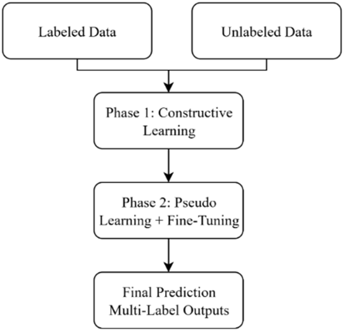
The two-phase framework: contrastive pre-training on labeled and unlabeled data, then joint fine-tuning with pseudo-labels. Figure from Dewabharata et al. (2025), IEEE COMNETSAT.

The labels are not independent. In this dataset 86% of e-money documents co-occur with at least one other category, and the correlation between categories is extremely high — 0.97 to 0.99. That has two consequences. First, it makes the problem easier per label, because categories travel together and reinforce each other. Second, it makes the hardest metric — predicting the exact label set of a document — genuinely difficult, because getting four of five labels right still counts as wrong. Keep that tension in mind; it explains almost every result below.

Why Legal Text Is a Special Case

Two properties of this domain break the usual playbook.

You cannot augment the data. Data augmentation — replacing words with synonyms, deleting tokens, back-translation — is the standard way to stretch small text datasets and to build the positive pairs that semi-supervised methods like FixMatch and MixMatch depend on. But legal language is semantically fragile: swapping "wajib" (obligatory) for "sebaiknya" (advisable) changes a legal obligation into a recommendation.² In a compliance setting, that is not noise; it is a different fact. Augmentation is therefore not just unhelpful — it is unsafe.

You have almost no labels. Our dataset contains 1,254 regulatory documents, but only 223 are expert-annotated. The remaining 1,031 are unlabeled. That ratio — roughly one labeled document for every five unlabeled — is where semi-supervised learning (SSL) earns its keep: it lets us exploit the large unlabeled corpus without trusting it blindly.

Background

Multi-Label Classification Approaches

Methods for MLTC fall into two broad families. Problem transformation converts the multi-label problem into one or more single-label problems:

• Binary Relevance (BR) trains one independent binary classifier per label. Simple, but it ignores label correlations entirely.
• Classifier Chains (CC) train classifiers in a sequence, feeding each label's prediction into the next. This captures dependencies, but it suffers from error propagation and is sensitive to the order of the chain.

Algorithm adaptation extends a learning algorithm to handle multi-label targets directly — from the lazy, instance-based ML-kNN to deep models such as Graph Convolutional Networks (GCNs) that model structural dependencies between labels. The recurring theme is the same: the labels are correlated, and the more explicitly a method models that, the better it tends to do.

Semi-Supervised Learning and Confirmation Bias

Self-training — also called pseudo-labeling — is the most common SSL strategy: a teacher model labels the unlabeled data with confident predictions, and the model is retrained on those labels. Its failure mode is confirmation bias: mistakes get baked in and reinforced, because the model keeps training on its own errors. Regularization (mix-up, per-batch labeled sampling) and self-pretraining are common mitigations.

Contrastive Learning

Contrastive learning offers a self-supervised way to shape an embedding space: pull positive pairs (similar) together and push negative pairs (dissimilar) apart, optimized with the InfoNCE objective.³⁴ In a supervised setting, the label information tells you which pairs are positive — the idea behind Supervised Contrastive Learning.⁵ The appealing part for us is that pair construction needs no augmentation at all.

The Method

The framework has two phases, both built on the same IndoBERT-base encoder (indobenchmark/indobert-base-p1), with a linear classification head producing one output neuron per label.⁶ Phase 1 uses both labeled and unlabeled text to pre-train the encoder with contrastive learning, yielding an embedding space that is already semantically organized. Phase 2 applies pseudo-labeling to the unlabeled set and fine-tunes the classifier jointly on labeled data (supervised loss) and pseudo-labeled data (unsupervised loss).

Phase 1: Contrastive Pre-Training

The design question is what counts as a positive pair when each document has a set of labels rather than a single one. We compare three answers, illustrated in the figure below.

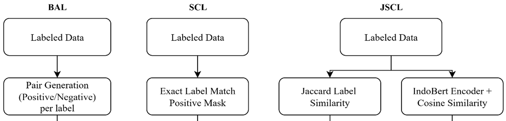
Contrastive learning strategies: (a) Binary Angular Learning, (b) Strict Supervised Contrastive Learning, and (c) Jaccard Similarity Contrastive Learning. Figure from Dewabharata et al. (2025), IEEE COMNETSAT.

Binary Angular Learning (BAL). BAL works over a predicted normalized angular distance $\theta$ between two samples and is adapted to the multi-label case by redefining the target from the label intersection:

• a pair is positive ($y=0$) if the two documents share at least one label;
• a pair is negative ($y=1$) if their label sets are disjoint.

${\mathcal{L}}_{\text{BAL}}=-\frac{1}{2}{\sum }_i[y_i\log {\theta }_i+(1-y_i)\log (1-{\theta }_i)]$

Minimizing this pushes samples related by at least one topic together while separating unrelated ones — a lenient definition of similarity that matches how regulatory topics overlap.

Strict Supervised Contrastive Learning (SCL). SCL is strict: a pair is positive only when the two documents share identical label sets. Given a batch, the objective follows the standard supervised-contrastive (InfoNCE) form:

${\mathcal{L}}_{\text{SCL}}={\sum }_{i\in I}\frac{-1}{|P(i)|}{\sum }_{p\in P(i)}\log \frac{\exp \left(z_i\cdot z_p/\tau \right)}{{\sum }_{a\in A(i)}\exp \left(z_i\cdot z_a/\tau \right)}$

where $z_i$ is the embedding of sample $i$, $P(i)$ is the set of indices whose label sets match $i$, $A(i)$ is the rest of the batch, and $\tau$ is a temperature that controls the sharpness of the distribution.

Jaccard Similarity Contrastive Learning (JSCL). BAL treats all overlapping pairs as equally positive and SCL treats only exact matches as positive. JSCL sits in between: it weights each positive by how similar the label sets are, using the Jaccard score. The cosine similarity in the embedding space is aligned with label similarity:

${\mathcal{L}}_{\text{JSCL}}=\frac{1}{B}{\sum }_{i=1}^B-\log \frac{{\sum }_{j\ne i}{w}_{ij}\exp \left(z_i\cdot z_j/\tau \right)}{{\sum }_{k\ne i}\exp \left(z_i\cdot z_k/\tau \right)}$

The weight $w_{ij}$ is the Jaccard similarity of the two label sets, normalized across the batch:

$w_{ij}=\frac{J_{ij}}{{\sum }_{k\ne i}{J}_{ik}},J_{ij}=\frac{|L_i\cap L_j|}{|L_i\cup L_j|+ϵ}$

where $L_i$ is the label set of document $i$ and $ϵ$ is a small constant that avoids division by zero. This is the strategy that best matches regulatory text: documents often overlap partially but meaningfully, and JSCL rewards the amount of overlap rather than treating it as all-or-nothing.

Phase 2: Fine-Tuning with Pseudo-Labeling

Once the encoder is pre-trained, the classifier is fine-tuned on a mix of ground-truth and pseudo-labeled data.

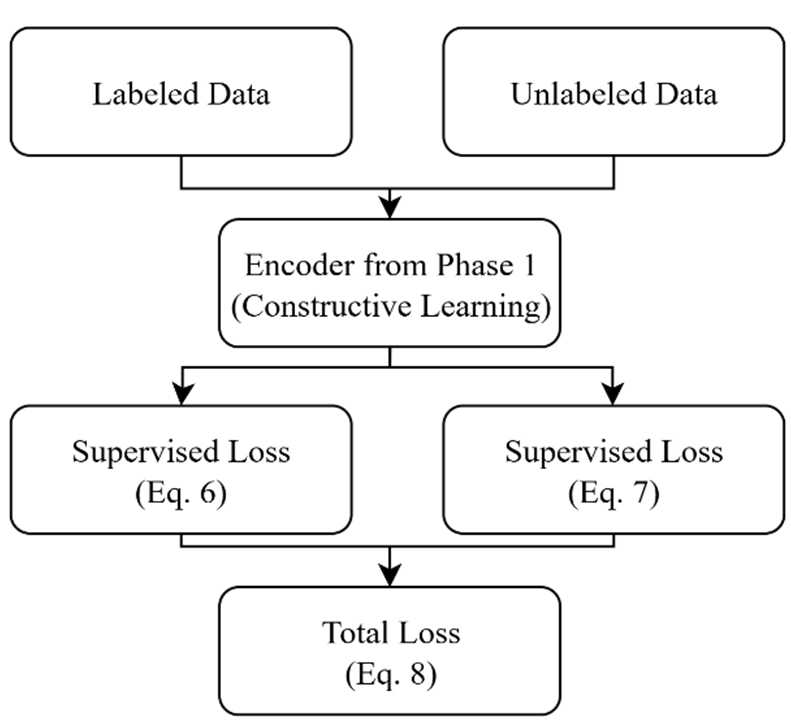
The second phase: supervised learning on the labeled set combined with an unsupervised loss on confident pseudo-labels. Figure from Dewabharata et al. (2025), IEEE COMNETSAT.

For each labeled document $x$ with ground-truth label vector $y$ and predicted probabilities $\hat{y}$, we add the supervised loss

${\mathcal{L}}_{\text{sup}}=\frac{1}{N}{\sum }_{i=1}^N\text{BCE}\left(y_i,{\hat{y}}_i\right)$

For each unlabeled document, the model generates a prediction, and only entries above a confidence threshold $\tau$ are kept as pseudo-labels $\tilde{y}$. This gating is what keeps bad pseudo-labels out:

${\mathcal{L}}_{\text{unsup}}=\frac{1}{U}{\sum }_{i=1}^{U}1\left[{\max }_k{\hat{y}}_{i,k}\ge \tau \right]\text{BCE}\left({\tilde{y}}_i,{\hat{y}}_i\right)$

The total objective is a weighted sum, where $\lambda$ controls how much the unlabeled data contributes:

${\mathcal{L}}_{\text{total}}={\mathcal{L}}_{\text{sup}}+\lambda {\mathcal{L}}_{\text{unsup}}$

The base architecture uses BCEWithLogitsLoss for per-label predictions, so each label is an independent sigmoid — which is also why the correlation problem remains: nothing in the loss explicitly models label dependencies.

Experimental Setup

Dataset

The corpus consists of Indonesian regulatory documents relevant to the financial technology industry, sourced from OJK and BI. Each entry concatenates the article body ("isi pasal") and its explanation ("penjelasan") into a single text input, with multi-label annotations over the five categories. It contains 1,254 documents: 223 labeled and 1,031 unlabeled, and is released publicly on Zenodo.⁷ The labeled subset was split 80/20 into training and validation using iterative stratification, which preserves the distribution of label combinations across both splits — critical in multi-label settings, where a naive split can leave rare label sets unrepresented.

The category counts are relatively balanced — e-money (100), credit card (96), QRIS (87), remittance (86), and payment gateway (84) — which reduces the risk of bias toward any single class. The 223 labeled documents produce 453 positive label assignments, confirming that most documents carry multiple labels.

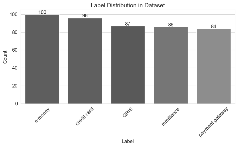
Label distribution: the five categories are relatively balanced. Figure from Dewabharata et al. (2025), IEEE COMNETSAT.

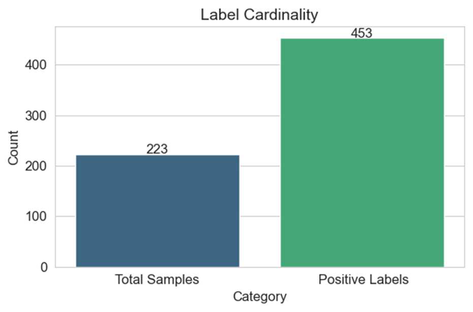
Label cardinality — most documents are associated with multiple categories. Figure from Dewabharata et al. (2025), IEEE COMNETSAT.

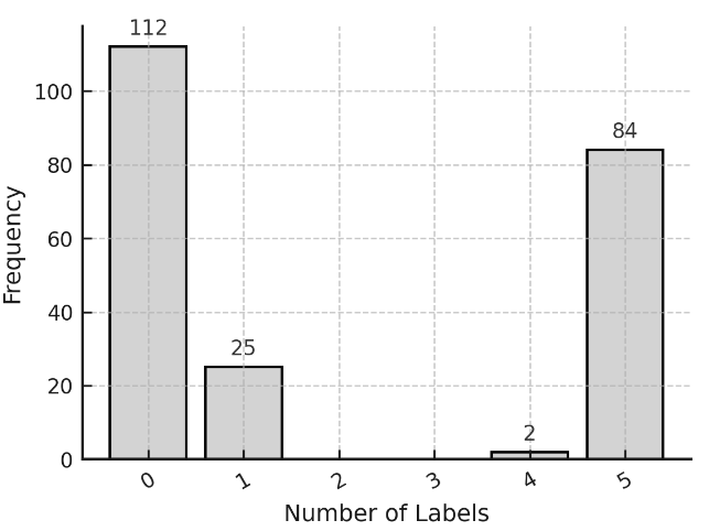
The distribution of exact label sets shows substantial heterogeneity. Figure from Dewabharata et al. (2025), IEEE COMNETSAT.

Training Configuration

All experiments ran on Python 3.11.9, PyTorch 2.1, and the Transformers library, on a single NVIDIA RTX 3080. The encoder was the same for all variants (~125M parameters, ~486 MB), with less than 0.5 MB of classification-head overhead.

Setting	BAL / SCL	JSCL
Contrastive warm-up	5 epochs	10 epochs (batch 16, lr 2e-5)
Optimizer	AdamW	AdamW
Learning rate	1e-5	encoder 1e-5, classifier 5e-5
Batch size	16	8 (plus 3-epoch linear probe at lr 5e-5)
Epochs	20	20
Regularization	dropout 0.4–0.5, L2 0.01	gradient clipping
Pseudo-label threshold	0.75	0.45
Unlabeled loss weight	$\lambda =0.5$	0.3, periodic pseudo-label updates
Pseudo-labeling	classifier confidence	k-NN with k = 11 random samples

JSCL uses a lower confidence threshold (0.45) because its k-NN-based pseudo-labels produce confidence distributions that are structurally different from the direct classifier probabilities in BAL/SCL; a higher threshold would starve it of training signal. Training took roughly 10–15 minutes per run, and inference averaged 0.2–0.3 seconds per article — fast enough for real-time use.

Evaluation Metrics

Because a single accuracy number hides everything interesting in multi-label classification, we report four averaging schemes.⁸

Macro average treats every label equally, regardless of how often it appears:

$F_{\text{macro}}=\frac{1}{T}{\sum }_{l=1}^T{F}_l$

Weighted average scales each label's score by its support $s_l$ (the number of true instances), so frequent labels count more:

$F_{\text{weighted}}=\frac{{\sum }_l{s}_l{F}_l}{{\sum }_l{s}_l}$

Micro average pools true positives, false positives, and false negatives across all labels before computing precision, recall, and F1:

$P_{\text{micro}}=\frac{{\sum }_{l}T{P}_l}{{\sum }_l(T{P}_l+F{P}_l)},R_{\text{micro}}=\frac{{\sum }_{l}T{P}_l}{{\sum }_l(T{P}_l+F{N}_l)},F{1}_{\text{micro}}=\frac{2P_{\text{micro}}{R}_{\text{micro}}}{P_{\text{micro}}+R_{\text{micro}}}$

Sample average measures whether the entire label set for a document was predicted correctly, averaged over documents:

$F{1}_{\text{sample}}=\frac{1}{D}{\sum }_{i=1}^{D}F1\left(y_i,{\hat{y}}_i\right)$

The gap between micro and sample averaging is the story of this paper: micro asks "did we find the individual categories?", sample asks "did we get the whole row right?".

Results

All numbers below correspond to the best-performing random seed.

Precision

Metric	SSL + BAL	SSL + SCL	SSL + JSCL
Micro-average precision	0.9570	0.9400	1.0000
Macro-average precision	0.9571	0.9410	1.0000
Weighted-average precision	0.9573	0.9232	1.0000
Samples-average precision	0.5050	0.5500	0.5333

Recall

Metric	SSL + BAL	SSL + SCL	SSL + JSCL
Micro-average recall	0.9889	0.9895	0.9440
Macro-average recall	0.9889	0.9909	0.9440
Weighted-average recall	0.9889	1.0000	0.9440
Samples-average recall	0.5250	0.5500	0.5244

F1

Metric	SSL + BAL	SSL + SCL	SSL + JSCL
Micro-average F1	0.9727	0.9641	0.9712
Macro-average F1	0.9726	0.9653	0.9711
Weighted-average F1	0.9727	0.9599	0.9711
Samples-average F1	0.5083	0.5500	0.5284

The headline result is strong: all three variants exceed 0.96 on individual-label F1, and BAL achieves the highest Micro-F1 at 0.9727, followed closely by JSCL (0.9712) and SCL (0.9641). JSCL reaches perfect Micro and Macro precision — zero false positives — which makes it attractive for compliance settings where a wrong flag is costly. The price is recall: JSCL trades away coverage, missing more relevant regulations. BAL and SCL lean the other way, prioritizing recall so that no relevant regulation is overlooked.

But then there is the sample average, and it tells a much more sober story. Despite per-label F1 above 0.96, sample-F1 sits between 0.51 and 0.55. The models are good at finding individual categories and poor at reproducing a document's complete label set. SCL is the best at this, which is a nice confirmation of its design: enforcing strict label-set alignment during pre-training preserves inter-label structure, so exact-set prediction improves even when Micro-F1 dips slightly.

Why Exact Sets Are Hard: Label Dependencies

The label analysis explains the gap. The co-occurrence matrix shows that 86% of e-money documents appear alongside other categories, and the correlation heatmap shows very strong positive associations among remittance, QRIS, and payment gateway.

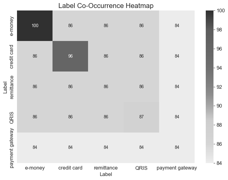
Label co-occurrence: regulatory topics are highly entangled. Figure from Dewabharata et al. (2025), IEEE COMNETSAT.

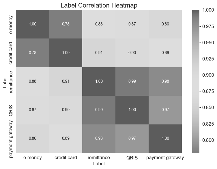
Label correlation heatmap: pairwise correlations reach 0.97–0.99. Figure from Dewabharata et al. (2025), IEEE COMNETSAT.

Indonesian regulatory texts typically address several interconnected services at once, so the label sets are structured, not random. A per-label sigmoid loss has no way to represent that structure — it can score each label well in isolation while still assembling the wrong combination. This is exactly the kind of dependency that graph-based encoders, correlation-aware losses, or structured prediction layers are designed to capture.

Statistical Rigor

To check whether the differences between methods are real, each experiment was repeated across 10 random seeds. The descriptive statistics for Micro-F1 tell an important story:

Model	Mean	Std	Variance	Min	Max
BAL	0.8951	0.0619	0.00383	0.7897	0.9727
SCL	0.8891	0.0493	0.00243	0.8173	0.9641
JSCL	0.8812	0.0497	0.00247	0.7742	0.9712

Standard deviations are small (0.05–0.06), so performance is stable — but the gap between the mean (~0.88–0.90) and the best seed (~0.96–0.97) is large. A paired t-test and bootstrap estimation confirm that no pairwise comparison is statistically significant (all $p>0.05$), and every 95% confidence interval spans zero:

Comparison	Δ mean	t	p (t-test)	p (bootstrap)	95% CI
BAL − SCL	−0.0059	−0.42	0.683	0.657	[−0.033, 0.019]
BAL − JSCL	−0.0139	−0.65	0.533	0.496	[−0.052, 0.027]
SCL − JSCL	−0.0080	−0.38	0.710	0.708	[−0.047, 0.030]

The interpretation is uncomfortable but honest: initialization variance dominates the choice of contrastive loss. All three strategies can reach strong results under a favorable seed, and which one "wins" depends as much on luck as on design. The most defensible conclusion is that IndoBERT's pre-trained representations contribute more to final performance than the specific contrastive objective — at this data scale.

Discussion

Putting it together:

• Per-label classification works well. Micro-F1 above 0.97 on best seeds shows the framework can reliably identify which regulatory categories apply.
• Exact-set prediction does not. Sample-F1 around 0.51–0.55 is the real bottleneck, and it is caused by the strong label interdependencies the per-label loss ignores.
• There is a genuine precision–recall tradeoff. JSCL is the precision-oriented choice (no false positives); BAL and SCL are recall-oriented (fewer missed regulations). The right pick depends on the cost of each error — in compliance, a missed obligation and a false alarm are not equally expensive.
• Algorithmic differences are within noise. With 10 seeds and no significant pairwise results, the contrastive loss function is not the lever that moves performance here.
• Augmentation-free SSL is viable but not sufficient. Avoiding augmentation is necessary for legal text, and pseudo-labeling does exploit the unlabeled corpus — but it does not solve the structural problem of correlated labels.

Takeaways and Future Work

The framework confirms that augmentation-free semi-supervised contrastive learning gives a strong foundation for regulatory text analysis, and that it can cut manual annotation cost and legal review time. But it also draws a clear boundary: learning individual labels is not the same as learning label structure.

The most promising directions follow directly from that boundary:

• Model label dependencies explicitly. Graph-based encoders (GCN-style), correlation-aware loss functions, or structured prediction layers can capture the co-occurrence and correlation patterns that a per-label sigmoid discards.
• Domain-adaptive pre-training. Continual pre-training on a regulatory corpus should improve representation quality specifically in this low-resource, high-jargon domain.
• Lean into the precision/recall asymmetry. A compliance pipeline could use the high-precision JSCL mode to propose labels and a recall-oriented mode to audit for misses, combining both under one human-in-the-loop review.

The broader lesson is one I keep running into: in real NLP systems, the interesting difficulty is rarely the average case. It is the structure — here, the fact that regulations come in entangled bundles — that separates a demo from something an auditor would trust.

References

1. A. Dewabharata, B. J. Santoso, M. I. A. Afiat, M. R. Ma'ruf, and M. Gosumolo, "Augmentation-Free Semi-Supervised Contrastive Learning for Multi-Label Classification of Indonesian Regulatory Texts," in 2025 IEEE International Conference on Communication, Networks and Satellite (COMNETSAT), Padang, Indonesia, 2025. DOI: 10.1109/COMNETSAT68601.2025.11324949
2. I. Chalkidis, E. Fergadiotis, P. Malakasiotis, and I. Androutsopoulos, "Large-scale multi-label text classification on EU legislation," in Proceedings of ACL, pp. 6314–6322, 2019. ACL Anthology
3. M. L. Zhang and Z. H. Zhou, "A review on multi-label learning algorithms," IEEE TKDE, vol. 26, no. 8, pp. 1819–1837, 2014.
4. J. Read, B. Pfahringer, G. Holmes, and E. Frank, "Classifier chains for multi-label classification," Machine Learning, vol. 85, no. 3, pp. 333–359, 2011.
5. M.-L. Zhang and Z.-H. Zhou, "ML-KNN: A lazy learning approach to multi-label learning," Pattern Recognition, vol. 40, no. 7, pp. 2038–2048, 2007.
6. Z.-M. Chen, X.-S. Wei, P. Wang, and Y. Guo, "Multi-label image recognition with graph convolutional networks," in Proceedings of CVPR, pp. 5177–5186, 2019.
7. Q. Xie, Z. Dai, E. Hovy, T. Luong, and Q. Le, "Unsupervised data augmentation for consistency training," Advances in Neural Information Processing Systems, vol. 33, pp. 6256–6268, 2020.
8. K. Sohn et al., "FixMatch: Simplifying semi-supervised learning with consistency and confidence," Advances in Neural Information Processing Systems, vol. 33, pp. 596–608, 2020.
9. E. Arazo, D. Ortego, P. Albert, N. E. O'Connor, and K. McGuinness, "Pseudo-labeling and confirmation bias in deep semi-supervised learning," in IJCNN, pp. 1–8, 2020.
10. P. Karisani and N. Karisani, "Semi-supervised text classification via self-pretraining," in Proceedings of WSDM, 2021.
11. A. van den Oord, Y. Li, and O. Vinyals, "Representation learning with contrastive predictive coding," arXiv:1807.03748, 2018.
12. T. Gao, X. Yao, and D. Chen, "SimCSE: Simple contrastive learning of sentence embeddings," arXiv:2104.08821, 2021.
13. P. Khosla et al., "Supervised contrastive learning," Advances in Neural Information Processing Systems, vol. 33, pp. 18661–18673, 2020.
14. T. Chen, S. Kornblith, M. Norouzi, and G. Hinton, "A simple framework for contrastive learning of visual representations," in Proceedings of ICML, 2020.
15. N. Lin, G. Qin, J. Wang, A. Yang, and D. Zhou, "An effective deployment of contrastive learning in multi-label text classification," arXiv:2212.00552, 2022.
16. F. Koto, A. Rahimi, J. H. Lau, and T. Baldwin, "IndoLEM and IndoBERT: A benchmark dataset and pre-trained language model for Indonesian NLP," arXiv:2011.00677, 2020.
17. M.-R. Amini, V. Feofanov, L. Pauletto, L. Hadjadj, É. Devijver, and Y. Maximov, "Self-training: A survey," Neurocomputing, vol. 616, p. 128904, 2025.

Citation

If you want to reference this note:

Ma'ruf, Muhammad Rifqi. "Teaching a Model to Read Financial Regulations." rifqimaruf.dev (2026). https://rifqimaruf.dev/writing/teaching-a-model-to-read-financial-regulations/

Footnotes

1. A. Dewabharata, B. J. Santoso, M. I. A. Afiat, M. R. Ma'ruf, and M. Gosumolo, "Augmentation-Free Semi-Supervised Contrastive Learning for Multi-Label Classification of Indonesian Regulatory Texts," in 2025 IEEE International Conference on Communication, Networks and Satellite (COMNETSAT), Padang, Indonesia, 2025. DOI: 10.1109/COMNETSAT68601.2025.11324949 ↩

2. This linguistic sensitivity is the core motivation for going augmentation-free. The framework instead defines positive and negative pairs directly from label information and patterns already present in the data. ↩

3. A. van den Oord, Y. Li, and O. Vinyals, "Representation learning with contrastive predictive coding," arXiv:1807.03748, 2018. ↩

4. T. Gao, X. Yao, and D. Chen, "SimCSE: Simple contrastive learning of sentence embeddings," in Proceedings of EMNLP, 2021. ↩

5. P. Khosla et al., "Supervised contrastive learning," Advances in Neural Information Processing Systems, vol. 33, pp. 18661–18673, 2020. ↩

6. F. Koto, A. Rahimi, J. H. Lau, and T. Baldwin, "IndoLEM and IndoBERT: A benchmark dataset and pre-trained language model for Indonesian NLP," arXiv:2011.00677, 2020. ↩

7. Sample labeled and unlabeled data: https://doi.org/10.5281/zenodo.17224158. ↩

8. C. D. Manning, P. Raghavan, and H. Schütze, Introduction to Information Retrieval. Cambridge University Press, 2008. ↩