Exploring Spatio-Temporal Cellular Traffic in Milan
- Spatio-Temporal
- Graph Neural Networks
- Telecom
- Data Exploration
- Machine Learning
When you first open a cellular network dataset, it looks like an ordinary time-series table: timestamps, cell IDs, and user activity counts.
| Timestamp (CET) | Cell ID | Internet (CDR) | Calls (CDR) | SMS (CDR) | Total Activity () |
|---|---|---|---|---|---|
| 2013-11-04 00:00 | 5161 (Duomo) | 4,821.4 | 78.2 | 214.5 | 5,114.1 |
| 2013-11-04 00:00 | 5262 (Centrale) | 2,912.8 | 45.1 | 138.4 | 3,096.3 |
| 2013-11-04 00:00 | 4654 (Perimeter) | 824.2 | 12.3 | 41.6 | 878.1 |
| 2013-11-04 01:00 | 5161 (Duomo) | 2,740.1 | 34.5 | 112.0 | 2,886.6 |
| 2013-11-04 01:00 | 5262 (Centrale) | 1,842.0 | 22.8 | 75.4 | 1,940.2 |
| 2013-11-04 01:00 | 4654 (Perimeter) | 481.5 | 6.2 | 22.6 | 510.3 |
Table 1. Sample hourly cellular telemetry from the Milan core network.
In telecom engineering, capital allocation carries severe asymmetric risk. Deploying a Small Cell infill costs ~€25,000; upgrading a Macro Sector costs ~€55,000.1 Under-provisioning during peak hours causes radio congestion and subscriber churn; over-provisioning strands capital on idle base station hardware.
Before designing complex forecasting models, the essential starting point is understanding the underlying characteristics and behavior of cellular telemetry. This post summarizes exploratory findings from Milan's urban core, four empirical realities behind cellular demand, and benchmark evaluations of standard baseline models.
Why Choose the Milan 2013 Dataset?
Granular, continuous metropolitan cellular telemetry is virtually impossible to obtain publicly. Following strict data privacy laws like GDPR, operators classified antenna-level Call Detail Records (CDR) as sensitive personal metadata and proprietary commercial intelligence.
Consequently, the Telecom Italia Big Data Challenge dataset (Milan, 2013) published by Barlacchi et al. (2015)2 remains the canonical "MNIST / ImageNet" benchmark for spatio-temporal telecom research.3
The original dataset spans an entire metropolitan province covering 10,000 grid cells. However, because peripheral outskirts exhibit low, unchallenging demand, this analysis focuses specifically on the 100 urban core cells.
This contiguous grid covers Milan's most congested activity centers—including the Piazza del Duomo cathedral, Milano Centrale railway terminal, and the San Babila commercial district—monitored continuously over 35 consecutive days (840 hours, November 4 – December 8, 2013).
Exploratory Findings
Metropolitan cellular traffic is governed by physical propagation and human mobility. Treating rows as Independent and Identically Distributed (I.I.D.) samples collapses under four empirical realities:
1. Heavy Tails and Leakage-Free Scaling
The raw activity distribution exhibited severe positive skewness (kurtosis ). The vast majority of observations cluster densely below 2,500 interaction units, but the distribution features an extreme heavy right tail exceeding 18,000 units during metropolitan rush hours (Figure 1A).
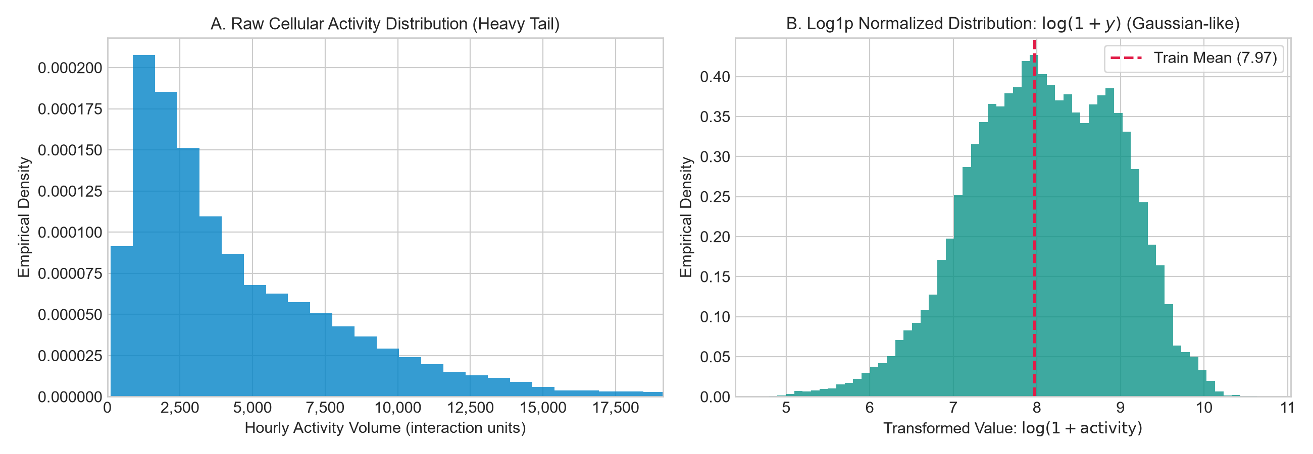
Figure 1. Distribution of 84,000 cellular traffic observations across the Milan core. (A) Heavy-tailed raw counts. (B) Gaussian-like density after transform.
Training directly on raw counts caused gradient instability: squared-error loss became entirely dominated by rare peak outliers, while off-peak baseline demand was virtually ignored. Applying a transform stabilized the variance into a quasi-Gaussian distribution (Figure 1B).
The Leakage Trap: When standardizing via Z-score (), computing and over the full 35 days leaks future test distribution into training. In this pipeline, parameters () were computed strictly on Weeks 1–3 (hours 0–503), leaving Weeks 4 and 5 unobserved during scaling.
2. Urban Functional Archetypes
Aggregating the city into a global average conceals radical micro-geographic divergence. Isolating individual cells across 168 consecutive hours (one week) reveals distinct functional archetypes (Figure 2):
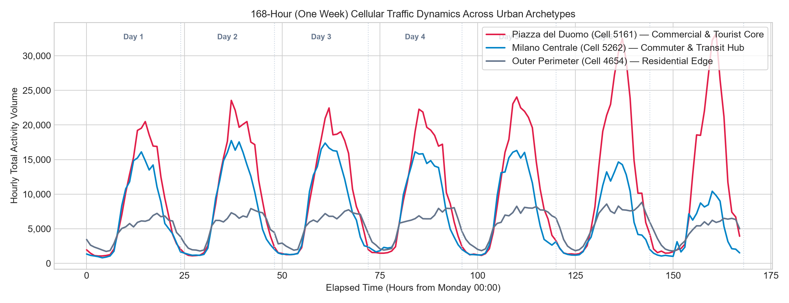
Figure 2. 168-hour demand profiles across three distinct urban archetypes.
- Piazza del Duomo (Cell 5161): High baseline activity, midday tourist/commercial peaks reaching 16,000 units, and sustained late-night weekend activity.
- Milano Centrale (Cell 5262): Sharp, punctual commuter spikes — morning arrivals (08:00–10:00) and evening departures (17:30–19:30).
- Outer Perimeter (Cell 4654): Subdued residential profile with narrow peak-to-trough amplitude.
3. Diurnal Dual Peaks and Weekend Phase Shifts
Plotting the average 24-hour cycle at Piazza del Duomo shows that weekdays and weekends follow fundamentally different dynamics (Figure 3):
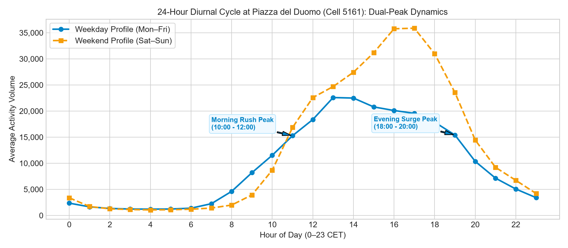
Figure 3. Diurnal profile at Piazza del Duomo: weekday dual peaks vs weekend gradual rise.
Figure 3 highlights this diurnal pattern clearly: activity drops to its daily baseline trough during early morning hours (02:00–05:00 CET) below 2,500 units. On weekdays (Mon–Fri), demand then surges into a clean dual-peak structure: morning business influx (10:00–12:00) and evening transit (18:00–20:00). On weekends, the morning peak vanishes; activity rises smoothly into late afternoon (15:00–17:00). A tabular model using simple lag features () predicting Monday morning from Sunday morning encounters catastrophic phase errors.
4. Spatial Concentration and Telecoupling
Demand is geographically concentrated along the Cadorna–Duomo–Centrale commercial axis (Figure 4). Outer cells experience less than 20% of core traffic volume.
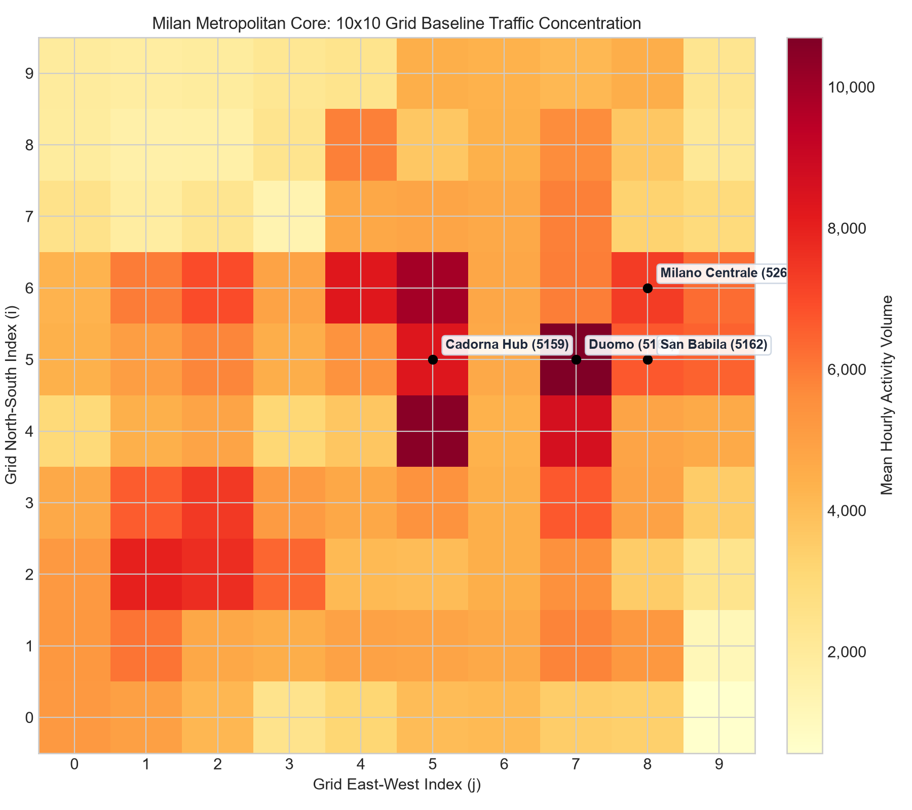
Figure 4. Baseline mean traffic across the 100-cell Milan urban core.
Crucially, physical distance does not tell the whole story. While a physical geographic graph (, thresholded Gaussian kernel at ) captures local RF spillover, certain distant cells correlate strongly despite having zero physical edge — a phenomenon known as telecoupling (Figure 5).
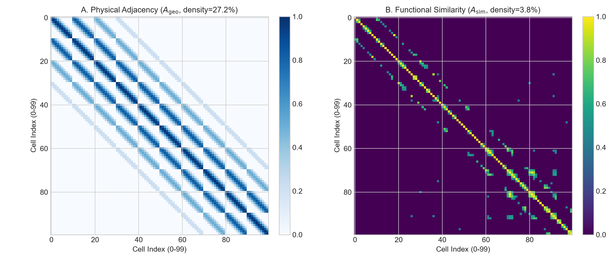
Figure 5. Adjacency matrices of the Milan core network: Physical geographic proximity () vs Detrended functional similarity ().
For a concrete example, index 26 (cell 4860) and index 91 (cell 5555) have centroids at (45.459332° N, 9.190054° E) and (45.474163° N, 9.175071° E). Their Haversine distance is approximately 2.02 km, and their detrended internet traffic has a training-set Pearson correlation of 0.437.
Look at row 26, column 91 in Figure 5, or the mirrored position. Panel A assigns zero weight because the distance exceeds the geographic graph's 0.75 km cutoff. Panel B retains a weight of approximately 0.437. This pair illustrates similar traffic patterns without a geographic edge; the correlation does not establish a commuter-related cause or identify the cells as railway stations.
Where Research Stands Today
Telecom traffic forecasting has evolved through three distinct eras:
- Classical Time Series (2000–2015): ARIMA, SARIMA, and Holt-Winters.4 Mathematically sound, but spatially blind — each cell is forecasted in isolation.
- Recurrent & 2D-CNN Models (2015–2018): ConvLSTM5 mapped cities onto 2D image matrices. However, urban geography does not behave like Euclidean pixel grids, and recurrent state transitions create severe sequential training bottlenecks.
- Spatio-Temporal GNNs (2018–Present): Graph WaveNet (Wu et al., 2019)6 combined Gated Dilated Temporal Convolutions (TCN) with graph diffusion and self-adaptive adjacency matrices, establishing state-of-the-art multi-step forecasting for cellular networks.7
Establishing Baseline Benchmarks First
Before leaping into complex deep learning architectures, good engineering discipline requires establishing solid benchmark baselines. Without clear baselines, there is no way to know whether the added computational complexity of a neural model delivers genuine predictive improvement.
To evaluate predictions on the held-out Week 5 test set ( urban core cells, 145 sliding windows across 24 forecasting horizons), I built three comparative baselines:
- Seasonal Naïve ( hours):
A deterministic benchmark that forecasts demand at hour using the observed value from the exact same hour one week prior (). Because commuter routines and weekend activities across Milan are highly repetitive, this deceptively simple model serves as a tough benchmark. - Historical Average (HA Weekly Profile):
Computes the empirical mean demand for each hour of the week (168 time slots) strictly over the training split (Weeks 1–3). Predictions rely entirely on these historical time-slot averages without short-term trend adaptation. - LightGBM Regressor (Tabular Gradient Boosting):
The industry-standard applied ML approach. Telemetry is flattened into tabular rows with engineered temporal lag features (), rolling statistics (12-hour and 24-hour mean and standard deviation), and cyclic calendar encodings (hour of day, day of week). Models are trained in a direct multi-horizon setting across each forecast step ().
Baseline Evaluation Results
Evaluating the three baselines across the held-out Week 5 test set yields clear performance characteristics:
| Baseline Model | Log-MAE | Log-RMSE | Activity MAE | Activity RMSE | WAPE (%) |
|---|---|---|---|---|---|
| LightGBM Regressor | 0.203 | 0.303 | 655.3 | 1,147.2 | 18.25% |
| Seasonal Naïve () | 0.225 | 0.364 | 634.8 | 1,062.9 | 17.68% |
| Historical Average | 0.230 | 0.371 | 679.0 | 1,126.3 | 18.91% |
Table 2. Benchmark performance of baseline models on the Week 5 test set (100 Milan urban core cells, hours).
Two key takeaways emerge from these baseline results:
- Short-Term Precision vs Periodic Stability: At the immediate 1-hour horizon (), LightGBM dominates with a WAPE of just 7.56% thanks to recent lag features (). However, as the forecasting horizon extends to 12 and 24 hours, the predictive power of short lags dissolves, pushing LightGBM's WAPE to ~20%. For extended horizons, Seasonal Naïve proves more resilient (18.83% WAPE at ) because pure weekly persistence avoids error compounding.
- Spatial Blindness: All three baseline models treat antenna cells as isolated silos. None capture RF propagation spillover from neighboring cells or the telecoupling dynamics uncovered during our exploratory analysis.
What Exploratory Analysis Taught Me
Reflecting on this exploratory and benchmarking phase, several foundational lessons stand out:
- What looks like a simple tabular dataset is fundamentally a dynamic spatio-temporal graph signal.
- Careless normalization leaks future distribution into training; strict temporal train splitting is non-negotiable.
- Physical distance alone does not dictate functional behavior: distant activity centers can move in lockstep (telecoupling).
- Tabular models like LightGBM excel at immediate short horizons, but weekly persistence (Seasonal Naïve) proves more stable over full 24-hour horizons.
In future notes, I will explore the PyTorch design of a Spatio-Temporal Graph Neural Network (ST-GNN) aimed at unifying spatial and temporal dynamics, and evaluate whether graph-based architectures can convincingly outperform these established baselines.
Footnotes
-
Capital expenditure benchmarks reflect heterogeneous network (HetNet) TCO models. See S. Tombaz et al., "Energy and Cost-Efficient Ultra-High-Capacity Wireless Access," IEEE Wireless Commun., vol. 18, no. 5, 2011; J. Markendahl and P. Werding, "A comparative study of deployment options, capacity and cost structure for macrocellular and femtocell networks," in IEEE BlackSeaCom, 2013; and Small Cell Forum (SCF), "Urban Small Cell Architecture and Economics," Document SCF106, 2015. ↩
-
A. Barlacchi et al., "A multi-source dataset of urban life in the city of Milan and the Province of Trentino," Scientific Data, vol. 2, p. 150055, 2015. DOI: 10.1038/sdata.2015.55 ↩
-
C. Zhang, H. Zhang, D. Yuan, and M. Zhang, "Citywide cellular traffic prediction based on densely connected convolutional neural networks," IEEE TMC, vol. 20, no. 4, pp. 1651–1665, 2021. ↩
-
G. E. Box et al., Time Series Analysis: Forecasting and Control, 5th ed. Wiley, 2015. ↩
-
X. Shi et al., "Convolutional LSTM network: A machine learning approach for precipitation nowcasting," in NeurIPS, 2015. ↩
-
Z. Wu, S. Pan, G. Long, J. Jiang, and C. Zhang, "Graph WaveNet for deep spatial-temporal graph modeling," in IJCAI, 2019, pp. 1907–1913. ↩
-
X. Wang et al., "Spatio-temporal analysis and prediction of cellular traffic in metropolis," IEEE TMC, vol. 18, no. 9, pp. 2039–2052, 2019. ↩