Flood Forecasting and Warning System

What if station locations, water-level history, and forecasts could be explored in one flow? That question shaped the Flood Forecasting Warning System (FFWS) dashboard. In this walkthrough, I share its features, design choices, and the work behind making the readings traceable.

The project is developed under a research program in the Department of Civil Engineering at Institut Teknologi Sepuluh Nopember. Its study areas cover the Welang River Basin in Pasuruan and monitoring locations in Surabaya. The dashboard is a monitoring and research prototype.

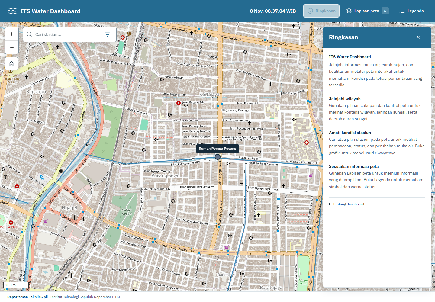
The local dashboard with the station map and summary panel. Sensor readings in these screenshots come from the local archive.

Meet the FFWS Dashboard

The feature screenshots below come from a local build using archived Surabaya readings. The values represent historical observations rather than live conditions. This build displays averages and minimum–maximum ranges; the centralized storage mode discussed later uses valid-sample medians for water levels. Interface labels in the screenshots are in Indonesian.

Choosing What to Show on the Map

The map is the main entry point. The Lapisan peta (map layers) panel controls station names, rainfall and water-quality information, administrative boundaries, and river networks. Users can also choose a basemap, from streets to satellite imagery. I keep these controls separate from sensor readings so users can first choose the geographic context they need.

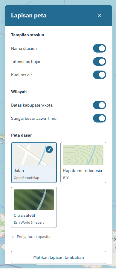
Layer controls stay in a side panel, leaving the main map available for exploration.

Finding a Station and Checking Its Status

When a station name is already known, search is faster than scanning the map. Typing “Pucang” returns Rumah Pompa Pucang together with its data status. In this example, Data terlambat means the readings are delayed, giving users context before they open the numbers.

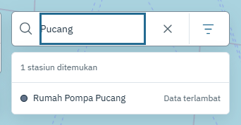
Search results pair each station name with its data-availability status.

Drawer Preview

Selecting a station moves the map to its location and opens a detail drawer on the right. Users can still see the relationship between the station, river, and surrounding area. For Pucang, the drawer offers two sensor channels, Pompa 1 and Pompa 2.

The example for Pompa 1 shows a sensor-to-water distance of approximately 342.3 cm. With a configured reference of 530 cm, the displayed water level becomes 187.7 cm, or roughly 35% of that reference. This percentage follows the sensor configuration; it does not represent stored water volume or the probability of flooding.

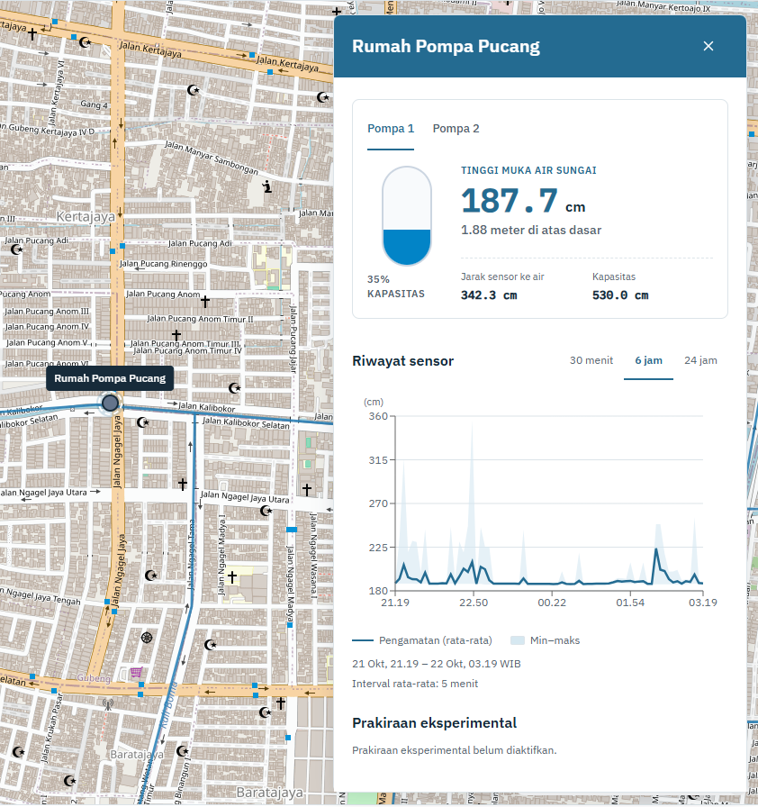
Location and sensor details remain side by side. These archived readings were last observed on October 22, 2026.

Exploring Changes in the Chart

The station page offers 6-hour, 24-hour, and 7-day ranges and a sensor selector. In the chart below, the horizontal axis shows time and the vertical axis shows water level in meters. The blue line represents average observations, while the light-blue band shows the minimum–maximum range within each aggregation interval.

That range reveals variation that a single average can hide. Breaks in the line show gaps in the available readings, rather than implying that water conditions were known throughout the entire period.

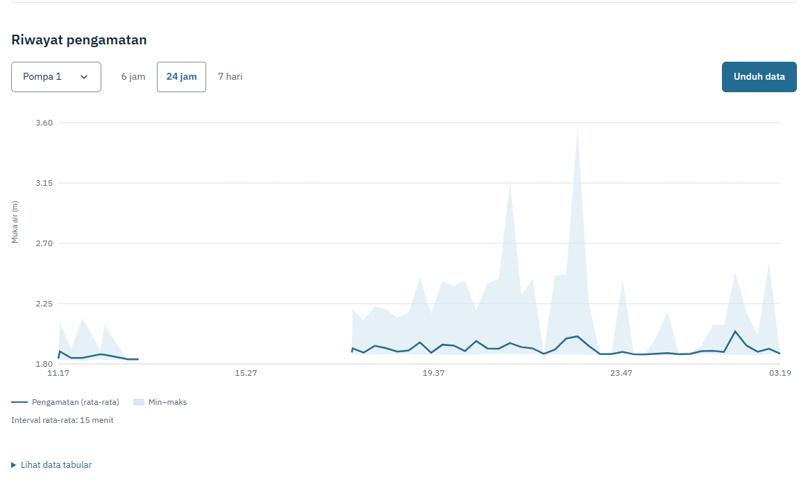
Pompa 1 over 24 hours. This archive build displays 15-minute averages with minimum–maximum ranges.

Downloading a Date Range

The Unduh data (download data) button opens start and end date controls. Users can take a period into Excel for further analysis without copying values from the chart. This screenshot shows October 21–22, 2026 selected; no export was submitted while capturing it.

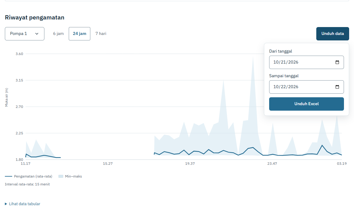
Date selection sits beside the chart to keep the transition from reading to analyzing data short.

In centralized storage mode, downloads separate observations from forecast history so model outputs are not mixed with measurements.

Reading Forecasts in Context

Forecast availability depends on configuration and data readiness. The centralized monitoring mode provides persistence and damped-trend baselines for one- to five-hour horizons. A preview based on the latest available history is distinguished from a forecast actually issued at its scheduled time.

The forecasting model uses an exponentially damped trend. I start with the latest water level and estimate its rate of change from the final hour within a six-hour input window. That rate is projected forward, with its influence gradually decreasing over the forecast horizon.

Here, $H_t$ is the latest water level, $b$ is the rate of change in cm per hour, and $h$ is the forecast horizon in hours. The parameter $\tau$ controls how quickly the trend fades; the current implementation uses $\tau =1$ hour. The final estimate is clipped between zero and the sensor reference height.

For example, a latest level of 200 cm and a rising trend of 10 cm per hour produce a one-hour forecast of approximately 206.3 cm. The model does not assume that the rise continues at a constant rate. Inputs are limited to water-level history from the same sensor; rainfall and upstream conditions are not yet included.

Behind the Scenes

The current frontend uses Next.js, TypeScript, MapLibre GL, and Recharts. Pages are exported statically, while monitoring data is requested from a FastAPI service. GeoJSON provides boundaries, river networks, and station locations.

Sensor MySQL sources / Welang history
                  ↓
          Data collection worker
                  ↓
     Supabase PostgreSQL → FastAPI
                              ↓
                   Dashboard + GeoJSON

A worker reads sensor sources in read-only mode and stores aggregates, source status, and forecast history centrally. The API still accesses raw samples for model inputs and downloads. Moving the API to another machine therefore does not require moving an entire local archive.

Water-level charts in this mode use the median of valid samples per five-minute interval. Checks cover timestamp completeness, sensor ranges, duplicates, and readings that remain unchanged for too long. The frontend receives both results and status from the API, keeping calibration rules out of browser-side calculations.

Further Reading

For the mathematical derivation, assumptions, and a worked example of the forecasting model, read An Exponentially Damped Water-Level Trend with Limited Data.